System of linear equations
Notation
| Symbol | Meaning |
|---|---|
| $\mathbf{F}$ | the field $\mathbb{R}$ or $\mathbb{C}$ |
| $V$ | a vector space over $\mathbf{F}$ (nonzero, finite-dimensional unless stated) |
| $\mathcal{L}(V,W)$ | linear maps $V \to W$ |
| $V/U$ | quotient of $V$ by a subspace $U$ |
The system as one equation
A system of $ m $ linear equations in $ n $ unknowns is a single equation
\[Ax = b, \qquad A \in \mathbf{F}^{m \times n},\ b \in \mathbf{F}^m.\]More generally, take $ T \in \mathcal{L}(V, W) $ and $ c \in W $ and ask for all $ x \in V $ with $ Tx = c $. Everything below is stated for $ T $; a system of equations is the case $ T = A $, $ c = b $.
There are two ways to read the equation, and each gives one picture of the solution set.
- Map view. Which vectors does $ T $ send to $ c $?
- Row view. Each row of $ A $ is one equation $ a_{i1} x_1 + \dots + a_{in} x_n = b_i $, and a solution must satisfy all of them at once.
The solution set
Structure of the solution set
Suppose $ T \in \mathcal{L}(V,W) $ and $ c \in W $. Then the solution set $ \{ x \in V : Tx = c \} $ is
- empty, if $ c \notin \operatorname{range} T $;
- the translate $ x_0 + \operatorname{null} T $, if $ c \in \operatorname{range} T $, where $ x_0 $ is any one solution.
If $ c \notin \operatorname{range} T $, no $ x $ satisfies $ Tx = c $. Otherwise pick $ x_0 $ with $ Tx_0 = c $. Then for $ x \in V $,
\[Tx = c \iff T(x - x_0) = 0 \iff x - x_0 \in \operatorname{null} T \iff x \in x_0 + \operatorname{null} T. \quad \blacksquare\]
general solution = particular solution + homogeneous solution
Here $ x_0 $ is the particular solution, and $ \operatorname{null} T $ is the solution set of the homogeneous system $ Tx = 0 $.
Existence and uniqueness
Both questions are answered by the theorem above. Existence is about $ c $, uniqueness is about $ T $.
| $ Tx = c $ has | exactly when |
|---|---|
| no solution | $ c \notin \operatorname{range} T $ |
| exactly one solution | $ c \in \operatorname{range} T $ and $ T $ is injective |
| more than one solution | $ c \in \operatorname{range} T $ and $ T $ is not injective |
In the last case there are infinitely many solutions, because $ \operatorname{null} T $ is a nonzero subspace.
Size of the solution set
Suppose $ V $ is finite-dimensional, with $ n = \dim V $ and $ r = \dim \operatorname{range} T $. By the fundamental theorem of linear maps, $ \dim \operatorname{null} T = n - r $. So a nonempty solution set is described by $ n - r $ free parameters, whatever $ c $ is.
The affine view
In the language of Affine Geometry, the theorem says that a nonempty solution set is an affine subspace of $ V $ with direction $ \operatorname{null} T $ and dimension $ n - r $.
Map view: changing $ c $ slides the solution set. The direction $ \operatorname{null} T $ does not depend on $ c $. So for a fixed $ T $, all the nonempty solution sets are parallel. Changing the right side moves the solution set without turning it, or makes it empty.
Row view: an intersection of hyperplanes. Each nonzero equation cuts out a hyperplane, and the solution set is the intersection of these $ m $ hyperplanes. Each equation that is independent of the others lowers the dimension by one, which gives $ n - r $ again, with $ r $ now read as the number of independent equations.
For two equations in $ \mathbb{R}^2 $, the hyperplanes are lines, and the three rows of the table above become three pictures:
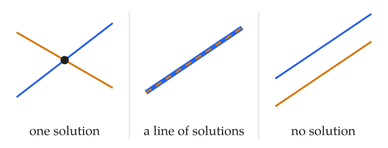
- One solution. The lines cross. The equations are independent, so $ r = 2 $ and the dimension is $ 2 - 2 = 0 $.
- A line of solutions. The lines coincide. One equation is a multiple of the other, so $ r = 1 $ and the dimension is $ 2 - 1 = 1 $.
- No solution. The lines are parallel and distinct. The left sides are multiples of each other but the right sides are not, so $ c \notin \operatorname{range} T $.
The quotient view
The translates of $ \operatorname{null} T $ are the elements of the quotient space $ V/\operatorname{null} T $. The theorem assigns to each $ c \in \operatorname{range} T $ exactly one of them, its solution set, and different $ c $ give different solution sets. This is the isomorphism
\[\tilde{T} : V/\operatorname{null} T \to \operatorname{range} T, \qquad \tilde{T}(x + \operatorname{null} T) = Tx,\]read backwards: solving $ Tx = c $ means computing $ \tilde{T}^{-1}(c) $.
The field of coefficients
If a linear system with all coefficients and constants in $\mathbb{Q}$ has a solution in $\mathbf{F} \supseteq \mathbb{Q}$, it has a solution in $\mathbb{Q}$.
Row-reduce the augmented matrix. Gaussian elimination uses only addition, subtraction, multiplication, and division by nonzero pivots. So starting from rational entries, every intermediate entry stays rational, and the resulting echelon form $R$ is rational.
The very same row operations are legitimate over $\mathbf{F}$ and produce the very same $R$. Now, if the system had no solution over $\mathbb{Q}$, the reduction would exhibit a row of the form $(0\;0\;\dots\;0 \mid c)$ with $c \neq 0$. But that row is equally an obstruction over $\mathbf{F}$, contradicting the existence of a solution there. So the reduction is consistent, and back-substitution (again only rational arithmetic) produces a solution with all $x_k \in \mathbb{Q}$. $\blacksquare$
Field-independent (determined over the small field $\mathbb{K}$): minimal polynomial, characteristic polynomial. Whether you compute it over $\mathbb{K}$ or over a bigger $\mathbf{F}$, you get the identical polynomial.
Field-dependent (can change when you enlarge): eigenvalues, eigenvectors, diagonalizability. These are about roots of polynomials, and roots can require a bigger field to exist.